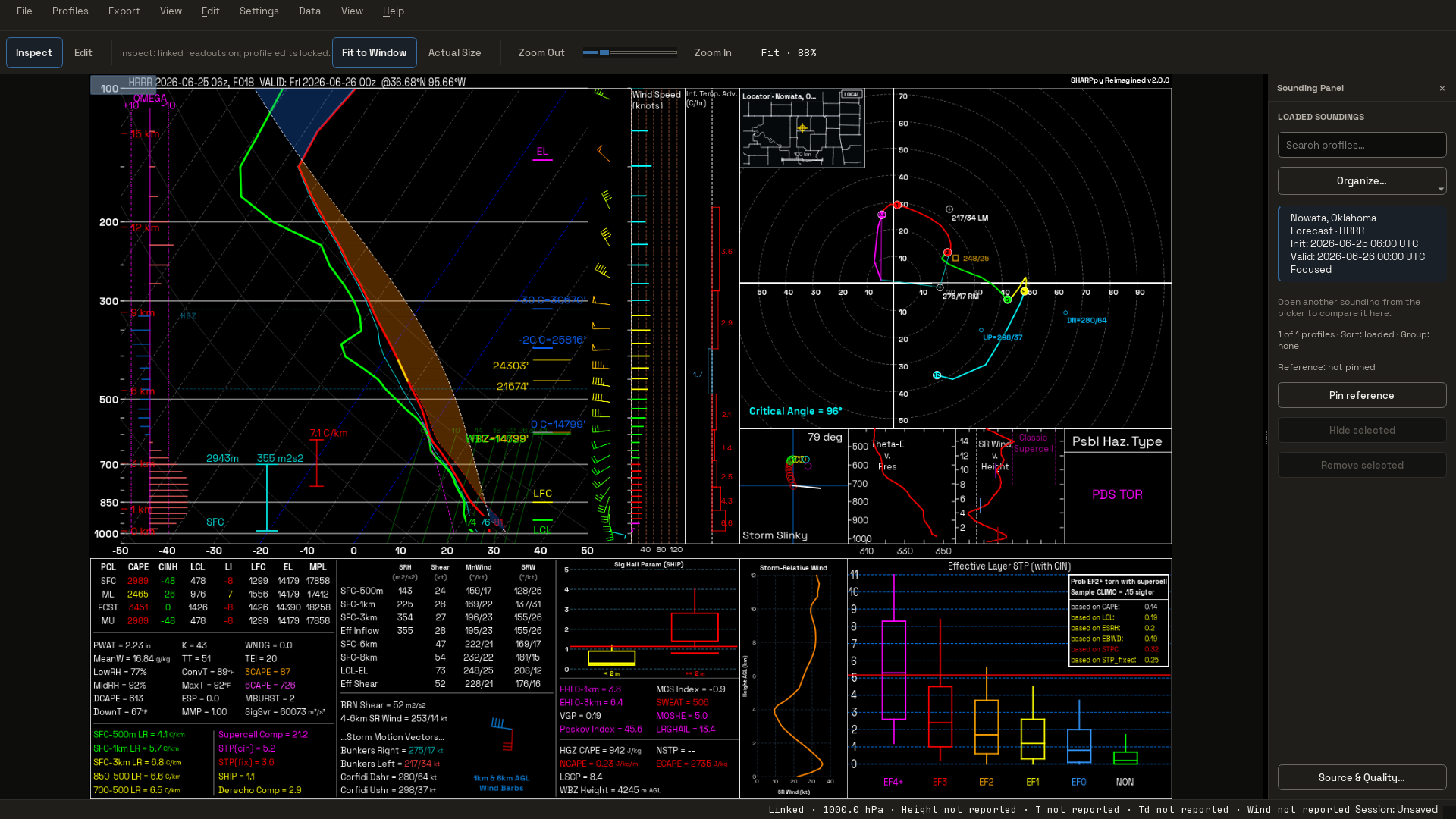
HRRR forecast point 36.68N 95.66W, F018, in the default Standard (dark)
palette with the Storm-Relative Wind chart selected. The locator inset combines
the SPC Day 1 categorical outlook (SLGT at the point) with the time-matched
HRRR Significant Tornado Parameter model-product field — rendered from
examples/soundings/hrrr_point_36.68N_95.66W_f018.npz.
SHARPpy Reimagined is a modernized, standalone fork of
SHARPpy, focused on packageable Python
3.11–3.13 workflows, Qt6/PySide6 rendering, and reproducible point-sounding
tools. It keeps the familiar SPC-style skew-T, hodograph, hazard, and
derived-parameter views while adding a redesigned desktop interface, clean
command-line entry points, bundled resources, and a test-backed
decoder/extractor layer.
Canvas palettes — light and colorblind modes (OAX 2014-06-16 19Z observed sounding)
Both palettes below render the same different sounding — the bundled OAX
observed profile — so the palette change is visible independently of the data.
Switch with File → Preferences (Standard / Inverted / Protanopia); the
choice persists across launches and applies to every panel and inset.
Inverted (light mode) — θ / θe Profile

Protanopia (colorblind mode) — Streamwiseness

All three captures were regenerated from 1.1.0. Together they demonstrate
three choices in the right-clickable chart slot: Storm-Relative Wind in the
Standard example above, θ / θe Profile in Inverted, and Streamwiseness in
Protanopia.
Contents
What's new in 1.1.0
Earlier releases sharpened the Skew-T. 1.1.0 builds the mesoanalysis around it,
so you can read the environment on the map, decide where the story is, and only
then pull a profile:
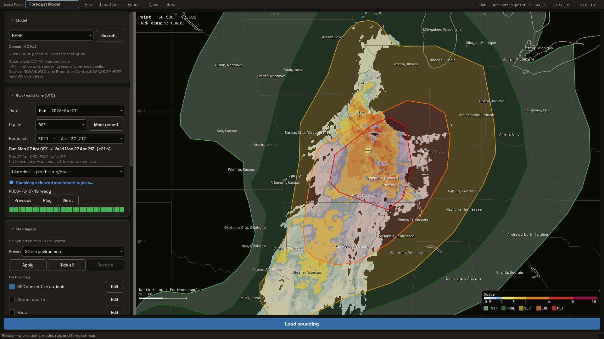
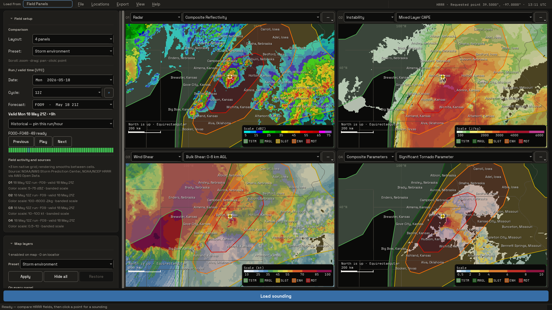
- Mesoanalysis fields on the picker maps. Map overlays → Show HRRR model
field paints any of 23 HRRR products across the map at the model's native
3 km, ordered the way a forecaster works down the scales. Open a sounding from
that map and the field you were reading follows it, at the same forecast hour.
- Area soundings: sample an airmass, not a point. Shift-drag a rectangle on
the Forecast Model map and the picker samples the model's own grid inside it.
Those samples are averaged into one sounding that opens in the ordinary
analysis window. Sample spacing is rounded up to a whole multiple of the
published grid spacing, so two soundings can never come out of one grid cell,
and the point count and download count are resolved before anything is
fetched. Winds average as components rather than as speed and direction,
moisture averages as mixing ratio rather than as dewpoint, and the mean starts
at the highest ground in the box.
- The parameter field. For the rarer question of where inside an area
something peaks, the box opens as a workspace instead: parameter maps,
ingredient screens that show where several thresholds hold at once, the same
area stepped through forecast time, and CSV or GeoJSON export. The new
box-extract command does the same from a terminal.
- Radar you can choose. Radar defaults to the single site nearest the map
centre and follows it as you pan, with the CONUS mosaic available as a
deliberate choice rather than the only option.
- A flat or curved map view. View → Map Projection switches every map tab
between the flat equirectangular view and a Lambert conformal conic that bows
its parallels and converges its meridians. Flat stays the default, and an extent
no cone can represent falls back to it. Every layer, imagery included, is
projected through the same transform.
- Lake shorelines. Inland water bodies — the Great Lakes among them — now have
outlines.
ne_50m_coastline carries only the ocean/land boundary, so lakes ship
as their own Natural Earth layer. Political boundaries are clipped to land, so no
border is ruled straight across open water.
- More on the sounding panels. The freezing level and wet-bulb zero are always
drawn on the Skew-T. The fire panel reports a ventilation rate; the winter panel
reports a Kuchera snow-to-liquid ratio and gives the dendritic growth zone in
pressure as well as feet. Every panel is now listed by name in the menu.
- Observed soundings from IGRA v2. Observed profiles can come from NOAA's
Integrated Global Radiosonde Archive, alongside the existing UWyo route.
The full list is in CHANGELOG.md.
Highlights
- Headless PNG rendering for
.npz, SPC tabular, BUFKIT, PECAN, and WRF-ARW
text sounding inputs.
- Portable
.npz point-sounding output from UWyo, the independent IEM RAOB
archive, ERA5, WRF-ARW, Herbie-backed forecast models, RRFS-A over NOAA
NOMADS, ECCC GeoMet, and Open-Meteo.
- Resumable multi-point/multi-hour jobs with one download per shared model hour,
bounded concurrency, atomic outputs, and a checksummed versioned manifest.
- A redesigned Qt6/PySide6 desktop application over the upstream SHARPpy widget
stack, with compatibility shims rather than forked widgets.
- A supported Rust-primary numerical and point-decoding backend, with an
independently optimized Python fallback and byte-level equivalence coverage
across the GRIB-decoding models. 19 public forecast products are configured;
see Configured models.
- A complete inverted/light sounding palette shared by the interactive GUI and
headless renderer, including contrast-aware labels and derived displays.
- Offline UWyo station catalog plus package-relative bundled fonts.
- Property-based pytest coverage for decoders, derived parameters, hazards,
renderer-facing widgets, and extraction paths.
Quick start
Requires Python 3.11, 3.12, or 3.13.
python scripts/install_sharppy_compat.py
sharpmod-render examples/soundings/hrrr_point_36.68N_95.66W_f018.npz out.png
sharpmod-render writes a 2x HD PNG by default; add --uhd for the larger
2.8x export or --lossless for the original-size compact/lossless PNG.
The installer hash-verifies the official SHARPpy==1.4.0a5 wheel, corrects
only its obsolete numpy==1.15.* requirement to this project's supported
range, records that provenance, installs the editable project plus render
stack, and requires pip check to pass. Use --source-wheel PATH for an
offline copy of the exact pinned upstream wheel.
For the full setup reference see installation.txt; for
usage recipes and Python API examples see docs/USAGE.md.
Desktop GUI
sharpmod-gui # or: python -m sharpmod.gui
On Windows, source-checkout GUI runs use Python 3.11–3.13. If this command is
invoked by Python 3.14 and the checkout has a .venv or .gribenv, the launcher
automatically hands the GUI to that compatible environment before Qt starts.
The packaged Windows release already bundles Python 3.11.
Loading a sounding
The Sounding Picker opens with five sources:
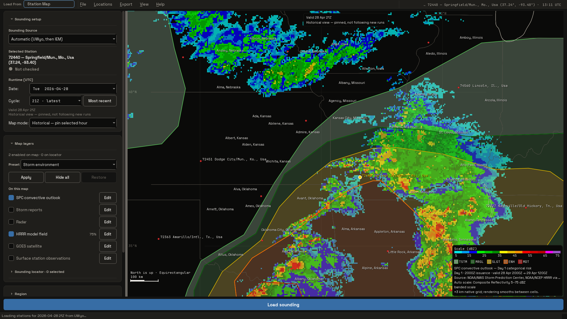
- Station Map — a clickable map of every UWyo radiosonde station over a
basemap of coastlines, lake shores, borders, and state lines. Click a dot to
select, double-click to open; scroll to zoom, drag to pan, pick a region from
the Map area menu, and choose a flat or curved view from View → Map
Projection. Observation
times are selectable every three hours from 00Z through 21Z.
- Station List — the full catalogue with live id/name filtering and the
same three-hourly UTC observation-time choices.
- Forecast Model — click a point or enter latitude/longitude, then choose a
public model, UTC run, forecast hour, and optional ensemble member. The picker
checks that inventory in the background. If publication is delayed, it offers
the newest available earlier cycle without silently changing the selection;
an uncertain check never disables manual Fetch. Timeline… queues a
selected range of as many as 72 hours into one viewer with a slider, playback,
step, and loop controls; completed hours remain available after cancellation
or a missing hour. Box… samples a whole area instead of one point — see
Box soundings.
- Reanalysis (ERA5) — choose any global point and hourly UTC analysis. The
picker previews the snapped 0.25-degree grid point, validates the optional
packages/CDS profile, caches completed point-hours, and keeps Qt responsive
while the synchronous CDS request runs in a worker.
- Open File — a local
.npz, SPC, BUFKIT, PECAN, or WRF-ARW text sounding
(or just drag the file onto the window). Its Raw WRF wrfout workflow
inspects a NetCDF domain/times in the background, validates a map point
against the actual curvilinear grid perimeter, then extracts and opens it.
Box soundings: an area at once
A point sounding answers "what does the atmosphere look like here". A box
answers "what does the airmass over this area look like". Hold Shift and
drag a rectangle on the Forecast Model map — or turn on Box… and drag
normally — and the picker samples the model's own grid inside it.
By default those samples are averaged into one sounding, which opens in the
ordinary analysis window like any other: same Skew-T, same hodograph, same
parcel logic, same outlook overlay, same town name. One gesture, one sounding,
one rendered image. Choosing Explore the box as a parameter field in the
confirmation dialog opens the area workspace instead, which answers the
different and rarer question of where inside the box something peaks.
What makes this trustworthy rather than merely fast:
- The model's resolution is respected. The sample spacing is rounded up to
a whole multiple of the product's published grid spacing, so two soundings can
never come out of one grid cell and no gradient is drawn between two copies of
the same number. Ask HRRR for 1 km spacing and you are told, in the plan, that
you are getting 3 km.
- One download, many soundings. Every point shares a model, run, forecast
hour, and member, so the whole box is a single field subset and one bulk decode
rather than N downloads.
- Every point is a real sounding. Each one goes through the same verified
surface contract as a single-point fetch: true surface pressure, terrain
height, and 2 m / 10 m values, with below-ground levels removed. No point is a
pressure ladder with an invented ground row.
- The cost is shown before it is paid. The confirmation dialog resolves the
lattice, spacing, point count, and number of downloads first, and the map draws
the exact points that will be sampled.
- Partial coverage stays honest. Points outside the model domain are kept in
the lattice and left blank instead of quietly reshaping the grid.
The box mean
Averaging soundings is easy to get wrong, so four things are done deliberately:
- Winds are averaged as components, never as speed and direction. The mean of
350° and 10° is 0°, not 180°. Every point is resolved to u and v, the
components are averaged, and the result is converted back.
- Moisture is averaged as mixing ratio, not as dewpoint. Dewpoint is
nonlinear in vapour pressure, so averaging it directly biases the column dry.
- The averaged dewpoint is clamped to the averaged temperature. Saturation
mixing ratio is convex in temperature, so the mean of several subsaturated
points can imply saturation at the mean temperature. Those levels are clamped
and counted rather than shipped as a supersaturated sounding.
- Only the layer every point shares is averaged. Terrain varies across a box,
so the points do not all start at the same pressure. The mean therefore begins
at the highest ground in the box, and the levels dropped at each end are
reported.
The result never pretends to be a point. The Skew-T's own title reads
HRRR box mean of 49, the window title says the same, an amber BOX MEAN
callout sits in the top-right of the plot itself, and the locator inset draws the
sampled rectangle and widens its view until that whole rectangle fits — so what
you see is the area the numbers came from, not a marker over a spot that was never
sampled on its own.
One caveat cannot be engineered away, so it is stated instead — in the dialog, in
the file's own metadata, and on the second line of that callout: the derived
parameters of the mean sounding are not the mean of the individual points'
parameters. CAPE of the average column is not the average CAPE. Averaging
smooths extremes, so a mean sounding describes the airmass — use the field
workspace when the extreme is the question.
Choosing the hour
The dialog opens on whatever forecast hour the sidebar has selected, so a box
follows the run you are already looking at. It is also a Forecast hour picker
in the dialog itself, listing every hour the product publishes, because changing
your mind should not mean cancelling, changing the sidebar, and drawing the
rectangle again. A mean is one hour by definition. In the field workspace the
optional hour sequence starts from whichever hour you picked here, and the offer
withdraws itself when you pick the last published hour, since there is nothing
after it to step through.
Drawing the box
Shift-drag always draws one. Turning Box… on makes a plain left-drag draw one
instead of panning, and while it is on the map still moves on a middle-drag or
right-drag — a selection mode that took the whole mouse away from you would be
a poor trade. A click without a drag stays a click: it moves the point rather
than committing a rectangle, and a few pixels of hand jitter will not commit one
either. Once a box is accepted the mode releases itself, so the next drag pans
again and you cannot accidentally start a second box on top of the one being
extracted.
The area workspace
Choosing the field mode instead gives you:
| Panel | What it answers |
|---|
| Field map | How a parameter varies across the area, coloured on the real basemap with per-cell values |
| Across the box | Min, mean, median, max, spread, and where the significant extreme is |
| Most significant 12 | A ranked list — jump straight to the most unstable or most sheared point |
| Ingredient overlap | Where every ingredient of a mode holds at once, and how much ground that covers |
Any cell opens as a complete Skew-T: double-click it on the map, or select it and
press Open sounding. Roughly 60 fields are available. The instability,
parcel-height, and kinematic fields are computed through the native backend and
resolve in well under a second for a full 256-point box; the SPC composites
(STP, SCP, SHIP, SHERBE, and the rest) need the full SHARPpy parcel surface at
about 0.4 s per point, so they are opt-in behind Add SPC composites and the
prompt quotes the expected wait.
Because the significant end of a field is not always the large end, the ranking
and the "extreme" readout follow the parameter: CAPE and shear rank downward,
while CIN, LCL, and LFC rank upward.
Ingredient screens
One field at a time answers "where is CAPE largest". A forecaster usually wants
"where are all of these true at once". The Ingredients picker hatches exactly
those grid points and reports how much of the box qualifies:
Ingredient overlap
MUCAPE ≥ 500 J/kg and 0-6 km shear ≥ 35 kt and 0-3 km SRH ≥ 100 m2/s2
34 of 90 points (38%), about 59,160 km²
Seven screens ship — surface-based storms, organized convection, supercell,
tornado ingredients, large hail ingredients, damaging wind ingredients, and
elevated convection. They are screening heuristics for narrowing attention, not
official products and not a forecast; every threshold is deliberately
permissive so a screen does not hide a marginal signal, and any of them can be
replaced with your own thresholds through the Python API.
The hatch uses the same visual grammar as the SPC outlook overlay on this map, so
it qualifies the cells it covers without hiding the field underneath. A point
that is missing one of the fields a screen needs is left blank rather than
shaded as unfavourable, and the count of such points is reported: an absence of
data never becomes a verdict.
What used to be under the field map
A pressure-versus-distance cross-section and a per-level spread band used to sit
below the field map. Both were vertical plots on a plain linear axis, which read
as broken next to this application's own Skew-T, and neither answered a question
the field map and the averaged sounding do not answer better. They are gone, and
the field map has the height back.
The numbers behind them remain: BoxAnalysis.vertical_transect() and
BoxAnalysis.envelope() still return the slice and the per-level band for a
script that wants to plot them its own way.
Boxes through time
Tick Step through forecast hours in the confirmation dialog and the same box
is sampled at up to twelve hours. The workspace gains a slider, step buttons, and
looping playback, so a field can be watched building and decaying rather than
inferred from two static hours.
Each hour is its own download — the saving a box gives you applies within an
hour, not across them — so the dialog states the hour count, the total sounding
count, and the number of transfers before anything is fetched. Jump to peak
goes straight to the hour whose extreme is the most significant, or, when a
screen is active, to the hour with the largest qualifying area. The field list is
the intersection across hours, so the selection cannot change under the slider.
Getting a box out of the app
Export saves the field map as a PNG exactly as drawn (legend and hatch
included), every point's values as CSV, or the sampled cells as GeoJSON for GIS.
The GeoJSON features are the sampled cells, not bare markers, because what
the model asserts is a value over an area of one grid spacing. A missing value is
an empty CSV field and an explicit null in GeoJSON — never a zero. A multi-hour
box exports every hour into one file, with an fxx column.
Working with a sounding
Each sounding opens in the full interactive SPC window built on the upstream
SHARPpy widget stack, so everything in the
SHARPpy GUI guide
still works.
Editing and readouts
- Right-click the Skew-T for the readout cursor, Modify Surface, parcel
lifting, and reset.
- Click + drag temperature / dewpoint / wind points to edit the profile —
every index recalculates live.
- Double-click the lower-left inset to swap lifted parcels.
- Undo / Redo:
Ctrl+Z reverses profile, interpolation, and storm-motion
edits; Ctrl+Y reapplies them. Each viewer retains the latest 50 edits.
Hodograph
Defaults to Mean Wind centering with a 20%-tighter viewport.
Right-click selects Mean Wind, Normal, or Storm Relative centering, and
double-clicking the RM/LM markers sets the storm motion. The active profile
has coloured dots with 0.5, 1, 3, 6, 9, and 12 inside them, and the locator
inset names the active sounding location/town in its title.
Zoom and view
| Gesture / key | Effect |
|---|
| Scroll over the Skew-T or hodograph | Zoom that panel alone; up magnifies, down returns. Each panel zooms independently. |
| Ctrl+scroll | Zoom the whole sounding, anchored on the pointer. |
| Middle-button drag | Pan, when the image is larger than the window. |
Ctrl+0 | Fit to window, and stay fitted as it resizes. |
Ctrl+1 | Actual size (100%) — the sharpest view, since the canvas is drawn at this size and any other scale is resampled. |
Ctrl++ / Ctrl+- | Step zoom. |
| Zoom slider | Continuous 20–400%. |
F11 / Escape | Enter / leave full screen. |
Ctrl+B | Show or hide the sounding panel. |
F1 | The full in-app controls guide. |
Zooming a single panel stops at the normal view, so at the default, scrolling
that way does nothing — that is also the reset. There is no drag-to-pan inside a
magnified panel, because dragging edits the profile.
Keys: ← / → step in time, ↑ / ↓ change ensemble member, Space swaps focus,
I interpolates, C collects observed, W returns to the picker.
Panels and reports
- Sounding panel (
Ctrl+B) lists every loaded sounding and marks the
focused one, selects the ensemble member, and opens the source and quality
report.
- Data → Source & Quality Inspector… shows the provider/source route,
backend and decoder, cache status, level and missing-field counts, surface
vorticity provenance, and non-mutating QC warnings for the focused profile.
- File → Preferences switches the colour palette (Standard / Inverted /
Protanopia), units, and the parcel visualized by default when a Skew-T opens.
For what every displayed index means — its formula, the clamps applied in code,
its colour thresholds, and its literature reference — see the
sounding parameter guide.
Themes and palettes
The Inverted palette is a complete light theme. Applying it updates the
Skew-T, hodograph, locator, storm slinky, inset products, IndexBoard, and
Streamwiseness panels in one live configuration change, and switches the
application chrome to paper-light at the same time. Theme-dependent text,
rules, legends, and semantic annotations are contrast-adjusted for a light
canvas while plotted scientific values, units, and established dark-theme
colours remain unchanged. Headless rendering uses the same selected palette.
Analysis sessions
Use File → Save Analysis Session… (Ctrl+Shift+E) in a sounding window to
save every loaded sounding, the active profile, current profile/interpolation/
storm-motion edits, parcel selection, and viewer state. Open Analysis
Session… (Ctrl+Shift+O) is available from both the picker and sounding
window and restores the saved soundings together in one viewer.
Session files use the .sharpmod-session extension and a versioned, portable
JSON format; they do not execute code or embed source GRIB downloads. Forecast
download directories still follow the normal lifecycle and are deleted when
their original viewer closes.
Export
The sounding window's Export menu saves the current view:
- Export Image (HD PNG) (
Ctrl+E) — a 2x high-density image of the full
window, including the mounted derived-parameter panels, with a sensible
default filename (STATION_YYYYMMDDHHZ_hd.png) in your Desktop folder.
- Export Image (UHD PNG) — a larger 2.8x ultra-high-density image
(
STATION_YYYYMMDDHHZ_uhd.png).
- Export Image (Lossless PNG) — the original-size compact/lossless image
for smaller files (
STATION_YYYYMMDDHHZ_lossless.png).
- Copy Image to Clipboard (
Ctrl+Shift+C) — the same current view, ready
to paste into another app.
- Export Text (SHARPpy) — the focused profile as a text file that loads
back into the app.
The upstream File → Save Image / Save Text actions remain available too.
External Windows automation can use
pwsh -NoProfile -File scripts/copy-image-to-clipboard.ps1 IMAGE.png instead
of embedding DataObject, StringCollection, and System.Drawing.Image
construction inside a quote-sensitive inline pwsh -Command string.
Data management and persistence
File → Downloaded Data Library… browses, validates, reopens/re-extracts,
pins, deletes, or copies provenance for cached model data.
Locations → Manage Saved Locations… stores searchable named points, supports
versioned JSON import/export, and displays saved and recent points as map
markers. Only labels and coordinates are persisted.
GUI choices persist across launches, including temperature/wind/PWAT units,
palette, top/bottom readouts, default parcel, multi-sounding behavior, dismissed
tips, recent files, and last selections. On Windows they are stored in
%APPDATA%\SHARPpy Reimagined\settings.ini; set SHARPMOD_SETTINGS_PATH to
use a different INI file.
The ERA5 and raw-WRF source panels expose Add to active sounding window
directly. Leave it enabled, change the point or available time, and fetch again
to overlay several soundings; it stays synchronized with File → Add New
Soundings to Active Window.
Location naming and the locator inset
Forecast, ERA5, and raw-WRF points accept an optional Location/town label.
Named saved locations populate it directly. When it is blank, a bundled
52,818-entry U.S. Census place/town index resolves and persistently caches the
nearest title across the contiguous United States and D.C.; state polygons
prevent nearby Canadian, Mexican, Atlantic, and Gulf points from receiving a
U.S. name. The resulting name appears above the hodograph locator-map inset.
A rate-limited OpenStreetMap Nominatim request is only a fallback when the
bundled search has no result. Entering a label skips lookup entirely, and
SHARPMOD_GEOCODER_URL=off disables that fallback. Headless rendering resolves
generic labels such as HRRR 41.53N 88.39W through the same path. Names are
used only for the title; no town labels are drawn inside the locator map.
See the
Nominatim usage policy
and OpenStreetMap attribution, plus
the offline CONUS index notes. The locator's map
context comes from separately bundled, one-degree Census county-outline tiles;
it performs no live map request and loads only tiles around the sounding.
Command line tools
| Command | Purpose |
|---|
sharpmod-render | Render a sounding file to a PNG |
uwyo-sounding | List, search, and fetch University of Wyoming soundings |
observed-sounding | Fetch from UWyo with an explicit IEM RAOB fallback |
era5-extract | Extract an ERA5 point sounding to .npz |
model-extract | Fetch all pressure levels for a supported forecast-model point sounding |
model-batch-extract | Run a resumable multi-point/multi-hour model job |
box-extract | Sample a lat/lon box on the model grid and report its parameter fields |
wrf-extract | Extract a WRF-ARW point sounding to .npz |
sharpmod-rust-sync | Check, rebuild when needed, and verify the local Rust backend |
# Observed sounding: try UWyo, then the independent IEM RAOB archive
observed-sounding fetch 72357 "2024-05-20 00" --out oun.npz --render oun.png
# Render the mixed-layer parcel on the Skew-T (MU is the default)
sharpmod-render oun.npz oun_ml.png --parcel ML
# Reanalysis / local WRF point soundings
era5-extract "2024-05-20 00:00" 35.18 -97.44 era5.npz --render
wrf-extract wrfout_d01_2024-05-20_00:00:00 35.18 -97.44 wrf.npz --render
# Canadian point sounding through ECCC GeoMet (no full-grid download)
model-extract gdps 45.50 -73.60 montreal.npz --run "2026-07-22 00" --fxx 6
sharpmod-render --parcel accepts SFC, ML, FCST, MU, EFF, and
USER. Parcel keys are case-insensitive.
era5-extract retrieves all 37 pressure levels plus a colocated surface record
from the official Copernicus Climate Data Store API. Create a free CDS account,
accept both the ERA5 pressure-level and single-level dataset licences, and copy
the credentials shown on the
CDS API setup page into
$HOME/.cdsapirc before the first request. Public forecast models continue to
use Herbie and do not require CDS credentials.
Forecast-model extraction (model-extract)
Install the GRIB stack before fetching model data. Add the render stack and the
upstream SHARPpy runtime when --render is needed:
# Extraction only
python -m pip install -e ".[era5]"
# Extraction plus PNG rendering
python scripts/install_sharppy_compat.py --extras era5,render
Discover the installed CLI and check remote inventory before a large fetch:
model-extract --help
model-extract --list
model-extract gfs --probe --fxx 0
# Also download and open the pressure-level subset during the probe
model-extract gfs --probe --fxx 0 --open-subset
# Check recent completed cycles and fail until the verified ground contract
# is complete (useful for provider monitoring)
model-extract rrfs-a --probe --lookback-cycles 12 --require-surface-contract
Fetch a point sounding by model key, latitude, and longitude:
# Keep the portable .npz and its .json metadata sidecar
model-extract gfs 35.18 -97.44 gfs_oun.npz --fxx 0 --loc "Norman, OK"
# Select an exact UTC cycle and forecast hour
model-extract gfs 35.18 -97.44 gfs_oun_f006.npz --run "2026-07-14 00:00" --fxx 6
# Render to a named PNG; fetched GRIB/.npz/.json data is removed afterward
model-extract hrrr 35.18 -97.44 --fxx 0 --render hrrr_oun.png
# Omit the PNG name to use the generated point-sounding filename stem
model-extract hrrr 35.18 -97.44 --fxx 0 --render
# Select an ensemble member (GEFS defaults to c00)
model-extract gefs 35.18 -97.44 gefs_p01.npz --fxx 0 --member p01
If --run is omitted, the CLI chooses the most recent configured cycle at or
before the current UTC time; upstream publication can lag that cycle, so use
--probe, use --lookback-cycles, or pass an earlier --run when inventory is
not available. --require-surface-contract makes a probe fail until surface
pressure/height, 2 m thermodynamics, and both 10 m wind components are present,
and lists the missing components. Without --render, the .npz and .json
outputs remain. With --render, only the PNG remains. The GUI instead retains
fetched files until the sounding window closes.
The verified surface contract. Every forecast extraction requires true
surface pressure and terrain height, 2 m temperature/moisture, and 10 m wind.
Isobaric records whose pressure exceeds the selected point's surface pressure
are discarded, then the verified ground row is prepended. ERA5 retrieves the
matching single-level fields in a second colocated CDS request. A provider that
does not publish the complete surface contract fails explicitly instead of
emitting a pressure-only profile. The completed profile must also pass
monotonic-pressure/height, thermodynamic, and wind quality checks before it is
written.
Batch and multi-point extraction
model-batch-extract accepts heterogeneous points and forecast hours. Requests
with the same model, UTC run, forecast hour, and member share one decoded
model-hour lease, while different hours run with a bounded 1–4 worker pool.
Single-point hours retain the normal point/subregion route and its GUI-compatible
spatial cache key; multi-point hours fetch one reusable field subset and decode
all local-GRIB points with vector element reads. Every .npz and .json
sidecar is atomic. The checksummed manifest is also atomic, so rerunning the
same command validates and skips completed outputs.
{
"version": 1,
"requests": [
{"id": "oun-f000", "model": "gfs", "lat": 35.18, "lon": -97.44,
"run": "2026-07-14T00:00:00Z", "fxx": 0, "output": "oun/f000.npz"},
{"id": "ict-f000", "model": "gfs", "lat": 37.65, "lon": -97.43,
"run": "2026-07-14T00:00:00Z", "fxx": 0, "output": "ict/f000.npz"},
{"id": "oun-f006", "model": "gfs", "lat": 35.18, "lon": -97.44,
"run": "2026-07-14T00:00:00Z", "fxx": 6, "output": "oun/f006.npz"}
]
}
model-batch-extract job.json --output-dir batch-output --workers 2
The Python API is sharpmod.batch_extract.run_batch(...); it accepts ordered
BatchRequest values and returns ordered per-request results plus completed
NPZ paths. Call BatchExtractor.cancel() for cooperative cancellation.
Pass an existing ModelHourCache as model_hour_cache= when a GUI or service
owns a longer-lived cache; the batch runner leases it but does not clear it.
Area extraction (box-extract)
box-extract is the scriptable form of the GUI's box soundings. It takes two
opposite corners, samples the model grid between them, and prints the resulting
parameter fields.
# What would this cost? Resolve the lattice without downloading anything.
box-extract hrrr 34.0 -99.0 37.0 -95.0 --dry-run
# Extract, then print area statistics and the MUCAPE grid
box-extract hrrr 34.0 -99.0 37.0 -95.0 \
--output-dir box-output --target-points 64 --field mucape
# Add the SPC composites and export every point to CSV
box-extract hrrr 34.0 -99.0 37.0 -95.0 \
--output-dir box-output --composites --csv box.csv
# Every available field key, with the expensive ones marked
box-extract --list-fields
Sampling density is set by either --target-points (aim for roughly this many)
or --spacing-km (request this spacing); both are rounded up to a whole multiple
of the model's grid spacing, and both are coarsened further if the box would
exceed the point budget. Every adjustment is reported in the plan rather than
applied silently:
Model HRRR (hrrr)
Box 34.00N-37.00N, 99.00W-95.00W
Size 363 x 334 km
Lattice 9 x 10 = 90 points (90 in domain)
Spacing 42.0 km (native 3.0 km)
Downloads 1
Longitudes may be given unwrapped to describe a box across the antimeridian:
box-extract gfs 50 170 56 190 is a 20-degree box through the dateline, not the
340-degree complement.
Three further options mirror the workspace:
# Where do all the supercell ingredients hold at once, and over how much ground?
box-extract hrrr 34.0 -99.0 37.0 -95.0 \
--output-dir box-output --screen supercell
box-extract --list-screens # every screen and its thresholds
# Step the same box through six forecast hours and report each one
box-extract hrrr 34.0 -99.0 37.0 -95.0 \
--output-dir box-output --hours 6 --hour-step 3 --field mucape
# Hand the sampled cells to GIS, tagged with the screen verdict
box-extract hrrr 34.0 -99.0 37.0 -95.0 \
--output-dir box-output --screen supercell --geojson box.geojson
--hours takes its hours from the model's own published cadence, so it cannot ask
for an hour the product does not publish. A sequence prints a per-hour table with
the peak marked, and --csv/--geojson write every hour into one file.
Exit codes are 0 success, 1 nothing extracted, 2 invalid arguments or an
unusable box, and 130 cancelled. The Python API is
sharpmod.box_sounding.plan_box_samples(...) plus
sharpmod.box_analysis.analyze_box(...); both are Qt-independent, so a script
and the desktop workspace cannot disagree about what a box contains.
Configured models
These are the canonical keys accepted by this checkout. model-extract --list
is the runtime source of truth and also reports known models that are not
enabled. Remote run availability still depends on the upstream provider.
| Canonical key | Model / product | Coverage | Configured forecast hours | Aliases / notes |
|---|
hrrr | HRRR pressure levels | CONUS | 00/06/12/18Z: F000-F048 hourly; other cycles: F000-F018 hourly | — |
rap | RAP 13 km AWIPS pressure levels | CONUS | F000-F051 hourly | — |
nam | NAM 12 km pressure levels | CONUS | F000-F084 every 3 hours | — |
nam-3km-conus | NAM 3 km CONUS nest | CONUS | F000-F060 hourly | nam3, nam-3km |
hrw-wrf-arw | NOAA HiResW WRF-ARW 5 km | CONUS | F000-F048 hourly | 00/12Z only; hiresw-arw, hrw-arw |
hrw-fv3 | NOAA HiResW FV3 5 km | CONUS | F000-F048 hourly | 00/12Z only; hiresw-fv3 |
rrfs-a | RRFS-A 3 km pressure levels | CONUS | F000-F084 hourly | 00/06/12/18Z only; rrfs; no omega; ~340 MB per model hour |
rrfs-a-alaska | RRFS-A 3 km Alaska nest | Alaska | F000-F084 hourly | 00/06/12/18Z only; rrfs-ak, rrfs-alaska |
rrfs-a-hawaii | RRFS-A 2.5 km Hawaii nest | Hawaii | F000-F084 hourly | 00/06/12/18Z only; rrfs-hi, rrfs-hawaii |
rrfs-a-puerto-rico | RRFS-A 2.5 km Puerto Rico nest | Puerto Rico | F000-F084 hourly | 00/06/12/18Z only; rrfs-pr, rrfs-puerto-rico |
rrfs-a-north-america | RRFS-A 13 km North America | North America | F000-F084 hourly | 00/06/12/18Z only; rrfs-na; cheapest RRFS domain covering CONUS |
gfs | GFS 0.25-degree pressure levels | Global | F000-F120 hourly, then every 3 hours to F384 | — |
cfs | CFS 6-hourly pressure levels | Global | F000-F384 every 6 hours | Member 1 by default |
ecmwf-ifs | ECMWF IFS Open Data | Global | 00/12Z: F000-F144 every 3 hours, then every 6 hours to F360; 06/18Z short cut-off stops at F144 | ecmwf, ifs |
ecmwf-aifs | ECMWF-AIFS Open Data | Global | F000-F360 every 6 hours | aifs |
openmeteo-icon-global | DWD ICON Global 11 km point profile | Global | F000-F078 hourly, then every 3 hours to F180; 06/18Z stops at F120 | icon, icon-global, om-icon; 12 measured pressure levels |
gefs | GEFS 0.5-degree pressure levels | Global | F000-F384 every 3 hours | Control member c00 by default |
gdps | Canadian GDPS 15 km point profile | Global | F000-F240 every 3 hours | 00/12Z; gem-global, cmc-global |
rdps | Canadian RDPS 10 km point profile | North America / Arctic | F000-F084 hourly | 00/06/12/18Z; gem-regional, cmc-regional |
Every product in that table was confirmed against live data to return a
sounding with a merged verified surface row. Products that cannot are withheld
from the picker and the CLI rather than offered and then refused; model-extract --list prints them with the measured reason. One is currently withheld:
| Canonical key | Why it cannot produce a sounding |
|---|
aigfs | AIGFS splits pressure and surface products, and its sfc product publishes only 2-m temperature, 10-m winds, and mean-sea-level pressure. Surface pressure, terrain height, and 2-m moisture are absent from every AIGFS product. |
Backends and performance
Rust-primary backend
Official Windows executables bundle the supported sharpmod_rs extension,
and the default auto mode uses Rust after validating its package version,
backend API, and required operations. The independently optimized Python
implementation remains a fully functional portable fallback, so source and
Python-only installations do not require Rust, Cargo, maturin, or a native
extension to run.
The native API accelerates standard kinematics, SB/MU/ML parcel summaries,
traced surface/forecast/MU/ML/effective and user parcel ascents, DCAPE, and
direct pressure-level GRIB point decoding. The GUI continues to expose
SHARPpy-compatible profile and parcel objects, with automatic Python-oracle
fallback if a native operation is unavailable.
To add the Rust backend to a source installation, first install a stable Rust
toolchain (Rust 1.88 or newer), then run these commands in the same Python
environment as sharpmod:
python -m pip install -e ".[rust-build]"
sharpmod-rust-sync
sharpmod-rust-sync --check
sharpmod-rust-sync rebuilds only when sharpmod_rs is missing or its version
does not match this checkout, then verifies forced-Rust selection in a fresh
Python process. --check is non-mutating; use --force after editing native
source. Extension developers can still run maturin develop --release --locked
directly from rust/sharpmod-rs.
Select the backend with SHARPMOD_BACKEND before starting the application:
| Value | Behavior |
|---|
auto | Default. Use Rust when it loads; otherwise use Python and record the fallback reason. |
python | Require the optimized Python implementation. |
rust | Require the Rust extension; report an error if it is unavailable or cannot load. |
Check the resolved backend without running a sounding workflow:
python -c "from sharpmod.backends import backend_info; print(backend_info())"
Rust is the supported primary backend when a compatible extension is present;
official Windows binaries include it. Standalone native wheels are still
CI/build artifacts rather than a separately published Python package. See the
Rust backend guide for source-build instructions,
fallback behavior, platform status, limitations, tests, and benchmarks.
Forecast-decoder performance and validation
Version 0.8.0 includes the two independently optimized GRIB implementations
introduced in v0.4.0. The Python backend reuses a file inventory and
nearest-point selection, reads only the required scalar fields, and keeps
bounded inventory, point-selection, and decoded-sounding caches. The Rust
backend memory-maps each local subset, iterates ecCodes messages without
copying the GRIB payload, and returns one NumPy-compatible matrix through a
single Python call. Neither implementation requires speculative parallel
decoding.
Both decoders understand GRIB multi-field messages in which one physical
message contains separate U- and V-wind fields. Their equivalence preflight
checks selected grid coordinates, pressure ordering, missing masks, and values
within field-appropriate floating-point tolerances. The matrix covers HRRR,
RAP, NAM, NAM 3 km, HRW WRF-ARW, HRW FV3, RRFS-A, GFS, AIGFS, CFS, ECMWF IFS,
ECMWF-AIFS, and GEFS.
Products without a published relative- or absolute-vorticity field can retain
the full xarray compatibility path in the production extractor so the
neighbor-wind vorticity estimate is preserved; their direct point decoder is
still measured separately and is not an end-to-end timing of that production
route. Optional fields published at a single pressure, such as GEFS omega, are
aligned only to that pressure and remain missing at other levels instead of
being broadcast through the sounding. Optimized Python and Rust return matching
pressure-aligned omega values and missing masks. The old/new GEFS benchmark
difference records the correction of the frozen legacy xarray full-column
broadcast; it is not a Rust availability gap.
See the all-model benchmark table,
its raw JSON record,
and the benchmark methodology. Network transfer is
excluded from decoder timings, and the JSON retains fixture hashes, raw
samples, selected coordinates, build fingerprints, and equivalence results.
Download acceleration and cache
The extractor keeps every pressure level published by the selected model while
avoiding fields that are duplicates for sounding construction. It tries the
smallest compatible route first:
- HRRR F000 analyses use direct point reads from the public HRRR Zarr archive
and normalize those columns straight into the compact decoder contract;
Canadian GDPS/RDPS query their six surface layers first, then request only
pressure layers above that ground pressure with bounded GeoMet fan-out.
- Indexed subsets at or below 32 MiB use validated, coalesced HTTP byte ranges
after selecting a healthy equivalent provider. Every indexed model uses up
to four bounded range workers by default. Large coalesced spans are split
into balanced fragments, with one session per worker, pinned object
identity, ordered atomic assembly, resumable fragments, and an automatic
sequential-range fallback. Live
RRFS and
all-model transport/decode
records retain timing and byte-equivalence evidence for that default.
- Larger HRRR, RAP, NAM, NAM 3 km, HRW WRF-ARW/FV3, GFS, CFS, and GEFS
transfers use a small NOAA NOMADS geographic subset; other indexed products
retain the range route.
- RRFS bypasses Herbie entirely and reads the published NOMADS
.idx
inventory itself, pulling both the prslev and 2dfld products over byte
ranges with eight workers by default. NOMADS offers RRFS no geographic
subset, so a field plan costs its full domain footprint; the combined
payload is cached per model hour and a provenance sidecar lets a repeat
request skip the network. See USAGE for the per-domain cost.
- Any unavailable or incompatible optimization falls back automatically to
the standard Herbie download path.
Local GRIB files decode directly into compact NumPy columns. Products without
a pressure-level vorticity field use a four-neighbor U/V stencil read directly
from two GRIB messages instead of opening xarray wind cubes. Multi-point batch
jobs vectorize both the sounding columns and those stencils, so each selected
message is unpacked once for all requested points; this is vectorized I/O, not
unsafe decoder threading.
The GUI keeps downloaded model hours under
%LOCALAPPDATA%\sharpmod\model-cache on Windows (or the platform cache folder),
up to 3 GB and 48 hours by default. In the File menu, Prefetch Next Forecast
Hour optionally warms the next valid hour, Clear Downloaded Model Cache
removes retained entries, and the model tab's Cancel button stops the active
request. Verified partial files from compatible range downloads are retained so
the same request can resume. Cache paths and metadata carry a contract version;
payloads produced by an older extraction contract remain visible in the data
library but are never reopened as current soundings.
Advanced overrides are available for testing or constrained environments:
| Environment variable | Default | Effect |
|---|
SHARPMOD_HRRR_BACKEND | auto | auto, zarr, or grib for HRRR F000 |
SHARPMOD_POINT_BACKENDS | auto | Set to grib to bypass point/subregion routes |
SHARPMOD_GRIB_DECODER | auto | auto uses direct point decoding with xarray fallback; direct requires it; xarray forces the compatibility path |
SHARPMOD_PROVIDER_RACING | 1 | Set to 0 to disable equivalent-provider probes |
SHARPMOD_RANGE_WORKERS | 4 | HTTP range-request workers for indexed models, clamped to 1-8; decoder execution remains serial |
SHARPMOD_GEOMET_WORKERS | 4 | Concurrent ECCC GeoMet layer-point requests, clamped to 1-8 |
SHARPMOD_MODEL_CACHE | platform cache | Override the GUI model-cache directory |
SHARPMOD_MODEL_CACHE_GB | 3 | Maximum retained cache size in GiB |
SHARPMOD_MODEL_CACHE_HOURS | 48 | Maximum retained entry age |
Standalone executable (Windows)
A one-folder, no-Python-required build is produced with PyInstaller. Install
the checkout itself first so the freezer can validate and bundle matching
package metadata:
python -m pip install ".[render,era5,wrf]"
python scripts/install_sharppy_compat.py --sharppy-only
python -m pip install pyinstaller
pyinstaller packaging/sharpmod_gui.spec --noconfirm
The result is dist/SHARPpy-Reimagined/SHARPpy-Reimagined.exe. Set
SHARPMOD_ONEFILE=1 in the build environment for a single self-extracting
dist/SHARPpy-Reimagined.exe instead. The one-folder ZIP is the recommended
Windows download because it starts substantially faster; the release page
labels the one-file build portable and explains the startup tradeoff in prose.
The official release workflow builds and installs sharpmod_rs before
PyInstaller packages the executable, making Rust the auto backend in the
published application. For custom local builds, the spec collects a compatible
installed extension when present; otherwise it logs a warning and produces a
fully functional Python-fallback bundle.
Official releases first run the reusable test workflow against the exact source
commit, build with the direct dependency versions in
constraints/release.txt, and publish from a separate artifact-only job. Only
that final job receives GitHub contents: write permission. The build rejects
stale or in-tree release metadata, embeds FileVersion and ProductVersion
from sharpmod/_version.py, and verifies the source, Python metadata, Rust
module/metadata, frozen runtime, and PE fields all agree.
Verifying a download
The Windows executables are not code-signed, so Windows SmartScreen may warn
the first time you run one. Choosing More info → Run anyway is expected.
Two things are published alongside every release so a download can still be
checked:
SHARPpy-Reimagined--SHA256SUMS.txt — compare with
Get-FileHash -Algorithm SHA256.
- GitHub build provenance — verify with
gh attestation verify --repo ShianMike/SHARPpy-Reimagined, which ties
the artifact to the workflow run and commit that produced it.
Install extras and testing
| Extra | Installs | Use it for |
|---|
[render] | SHARPpy runtime companions | PNG rendering |
[era5] | CDS API, Herbie, cfgrib, ecCodes, xarray, numcodecs, pyproj | ERA5 and public forecast-model point extraction |
[wrf] | xarray, netCDF4 | WRF-ARW NetCDF extraction |
[dev] | pytest, Hypothesis, pytest-xdist, pytest-timeout, PyYAML | Test and workflow-validation work |
[quality] | Ruff, pip-audit, pytest-cov | Static checks, dependency audit, and coverage |
[rust-build] | maturin | Build the supported Rust backend locally (Rust toolchain installed separately) |
python scripts/install_sharppy_compat.py --extras dev,quality,era5,wrf,render
# Fast deterministic feedback with bounded, Qt-safe worker grouping.
python scripts/run_test_lane.py fast --workers 4
# Full 100-200-example scientific properties.
python scripts/run_test_lane.py property --workers 4
# Exact non-parallel release gate.
python scripts/run_test_lane.py serial-release
# Optional source-checkout Rust backend
python -m pip install -e ".[rust-build]"
sharpmod-rust-sync
Each lane checks its wall time against the versioned budget in
constraints/test-performance-baseline.json, which carries separate
github-actions limits because hosted runners are slower than the reference
machine. Hypothesis keeps an example database under .hypothesis/; a large
local cache inflates property-test timings on repeat runs.
Data flow
UWyo / ERA5 / WRF / public forecast models
|
v
portable .npz point sounding
|
v
sharpmod-render
|
v
SPC-style skew-T + hodograph PNG
Repository map
sharpmod/
gui.py interactive desktop app entry point
gui_picker.py sounding picker shell and source panels
gui_viewer.py sounding window: zoom, view controls, sidebar, help
theme.py Qt-free design tokens and chrome style-sheet generator
gui_theme.py applies the chrome theme to a QApplication
render.py headless PNG render entry point
box_sounding.py Qt-free area sampling: regions, grid-aligned lattices, budgets
box_analysis.py Qt-free fields, statistics, screens, envelopes, and sequences
box_mean.py Qt-free averaging of a sampled box into one sounding
box_export.py Qt-free CSV and GeoJSON writers for a sampled box
gui_box.py box extraction/analysis workers and the area workspace window
backends/ optimized Python/Rust kernels and direct GRIB point decoders
sharptab/ derived-parameter and meteorological calculations
io/ decoders for SPC, BUFKIT, PECAN, WRF-ARW, .npz, and UWyo
viz/ Qt6/PySide6 rendering widgets
tools/ UWyo, ERA5, forecast-model, WRF, basemap, and render CLI tools
resources/ bundled fonts, station catalog, and GUI basemap/icons
tests/ unit, smoke, and property-based tests
packaging/
sharpmod_gui.spec PyInstaller spec for the standalone GUI build
rust/sharpmod-rs/ supported PyO3/maturin backend extension crate
benchmarks/ Python-versus-Rust equivalence-first timing harness
examples/
example_sounding.png
soundings/ bundled sample inputs
docs/
USAGE.md workflow guide and API examples
RUST_BACKEND.md Rust-primary setup, fallback behavior, and limitations
Reference documents:
Attribution
This project builds on the abandoned upstream
SHARPpy project. See LICENSE
for the BSD 3-Clause terms and NOTICE for upstream attribution.